The bar I set for a model is that it should yield answers we believe to questions that matter. For a model of growth, the two questions that matter most are:

1. Speeding-up: Why has the rate of growth at the technological frontier been increasing over time?

2. Missed Opportunities: Why have so many countries that start from far behind the frontier failed to achieve rapid catch-up growth?

This month, I’m writing a series of posts in response to a nudge from Joshua Gans noting that this is the 25th anniversary of the publication of my paper Endogenous Technological Change, JPE (1990). In this post, I’ll recapitulate the evidence that convinced me when I was writing the 1990 paper that these are the two big questions that growth theory should address. In a subsequent post, I’ll explain why the conceptual framework that I used in the 1990 paper, one that relies on partially excludable nonrival goods, is the bare minimum for answering them.

My conviction that the rate of growth in GDP per capita at the technological frontier had to be increasing over time sprang from a simple calculation. Suppose the modern rate of growth of real GDP per capita (that is the growth rate after taking out the effects of inflation) is equal to 2% per year and that income per capita in year 2000 is \$40,000. If this rate had prevailed for the last 1000 years, then in the year 1000, income per capita measured in the purchasing power of dollars today would have been \$0.0001, or 0.01 cents. This is way too small to sustain life. If the growth rate had been falling over time instead of remaining constant, then the implied measure of GDP per capita in the year 1000 would have been even lower.

Figure 1

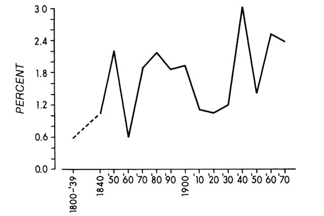
Figure 1 comes from my 1986 paper, which presented my ver 1.0 model of growth, the one I developed in my 1983 Ph.D. thesis. It shows the kind of data that I used to back up the simple calculation based on projecting back income in the past. (The source for these data was a 1979 article by Angus Maddison that was published in Kyklos.)

Table 1

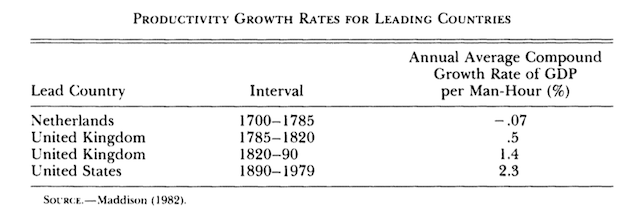
Table 1 shows the evidence I used in an attempt at going even farther back in time and which recognized that technological leadership had shifted between countries over time. (The source for these data was a book that Maddison published in 1982.)

Figure 2

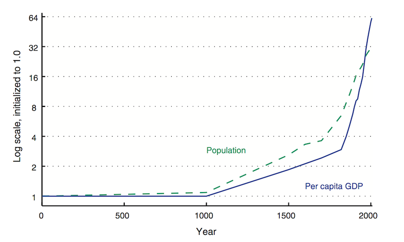
Figure 2, which is taken from a more recent paper with Chad Jones, gives a graphical presentation of the long view that draws on more recent Maddison data (from 2008.)  The numbers for population and GDP are totals for the area now occupied by the United States and 12 Western European countries. In this figure, the initial value of both population and GDP per capita are normalized to 1 in the year 0. Because the vertical axis is in logarithms, the slopes of the curves are growth rates. Both obviously increase over time.

According to this figure, GDP per capita today is about 64 times its value in the year 1000, not 500 million times larger, as it would have to be if the growth rate had been equal to 2% per year for 1000 years. These data also contradict another implication of a model with a constant, exogenous rate of technological progress. In such a model, an increasing rate of growth of population would be associated with a falling rate of growth of GDP per capita.

Moreover, as Angus Deaton emphasized in his recent book, The Great Escape, this type of calculation underestimates the remarkable increase in the rate of improvement in standards of living because it takes no account of the rapid improvement in health in the modern era. Like Deaton, I look at these data and see grounds for optimism. In his forthcoming book The Rise and Fall of American Growth, Robert Gordon looks at the same evidence and concludes that the good times are over and that progress in the future will be slower.

Reasonable people can differ about what the future holds, but the simple calculation that first got me thinking about this (and which no doubt influenced how Maddison did the backward projections to come up with his estimates) leaves no room for doubt about what happened in the past. The rate of growth of GDP per capita has increased over time. The rate of progress in standards of living has increased even more.

Because the logic is so clear, there has never been any serious debate about the historical fact that is the basis for the question about speeding up. My contribution was merely to pose the question. How could economists understand in a conceptual framework that still built on the logic of diminishing returns based on resource scarcity that has been central to economic theory at least since the work of Malthus and Ricardo?

It is not enough to say “_________ explains why Malthus was wrong,” and to fill in the blank with such words as “technological change” or “discovery” or “the Enlightenment” or “science” or “the industrial revolution.” To answer the question, we have to understand what those words mean. As I’ll argue, there is no way to understand those words without understanding the more fundamental words “nonrival” and “excludable.”

The other striking fact about growth emerged from the Heston-Summers data for many countries that became available during the 1980s.

Figure 3

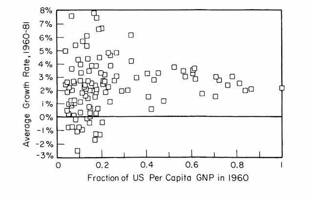
Figure 3 plots the real rate of growth of GDP per capita measured in local purchasing power, for a sample of countries over the interval 1960 to 1981. On the horizontal axis, it plots the ratio of real GDP per capita in 1960 of each country to real GDP per capita in the United States. The United States is the country on the upper edge of the graph, the one that starts in 1960 with a ratio of 1. (The figure is taken from a paper I published in 1989. As far as I know, this was the first instance of a plot of this type, one that reveals the “triangle” pattern in the data.)

The downward sloping upper boundary of the triangular cluster of points shows the behavior we would expect: Countries that start out far behind the frontier have faster rates of growth as they catch up with the frontier. Moreover, these rates of growth can be very fast. Some countries that started at less than 20% of US GDP per capita grew at rates that exceeded 6% per year. The key take away from this figure is that most poor countries did not take advantage of the potential for rapid catch-up growth that the frontier shows is possible. Holding constant the level of income in 1960, some other variable has a big effect on subsequent growth.

The second question, about missed opportunities, asks what that other variable might be. Once again, it is not enough to say that “many poor countries fail to take advantage of rapid catch-up growth because they ____________” and then fill in the blank with such words as “have bad institutions” or “are corrupt” or “lack social capital” or “are held back by culture.”

Back when we were first looking at these data, one common way to fill in the blank was to frame it the other way and say that “poor countries can achieve rapid catch-up growth only if __________” and to fill in the blank with “they are small.” At that time, the countries with the fastest growth rates,  the ones were referred to then as the “Asian tigers” – Hong Kong, Taiwan, South Korea, and Singapore – were indeed small. But of course, China was already making a remarkable transition to faster growth. To a lesser extend, so too was India. So the current generation of economists is more likely to say that fast catch-up growth is possible only for big countries.

This kind of over-confident, casual empiricism, undisciplined by any formal theory, is a sign that economists do not have a good answer to the second question.

Previous posts in this series:

#4: Economic Growth

#3: Clear Writing Produces Clearer Thoughts

#2: Human Capital and Knowledge

#1: Nonrival Goods After 25 Years

Thanks to Joshua Gans for spurring this series with his post here.